Fall 2024 CS 180 Project4

Fun With Diffusion Models!

By Yiyu Chen

Part A: The Power of DiffusionModels

0: Setup

In this Part, we use the DeepFloyd IF diffusion model, which was trained for text-to-image conversion. DeepFloyd has two stages. The first stage produces images of size 64 x 64 and the second stage takes the outputs of the first stage and generates images of size 256 x 256.

Sampling from the Model

For a better understanding of the model, here are the outputs of the model for the three provided prompts in different stages.

    prompts = [ 
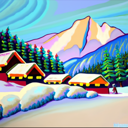
        'an oil painting of a snowy mountain village', 
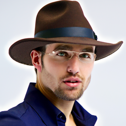
        'a man wearing a hat', 
        "a rocket ship", 
        ]

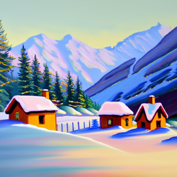
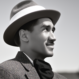
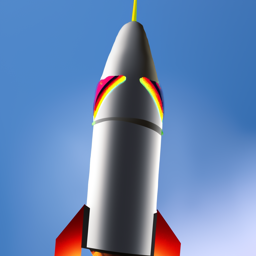
The above images are generated when num_inference_steps of both stage are set to 20

All of the generated image reflect their text prompts well. At stage1, the content of the images was already visible, indicating that the 64x64 images were already of reasonably good quality, even if they were small and simpler. After stage2 the images evolved to a more elaborate and visually appealing stage. Looking at them one by one, the final snowy village images lacks detail and looks a bit simple. The image of the man is the best one, with more realistic presentation. The image of the rocket is the simplest, basically just blocks of color and similar to a sketch even after it passed the stage 2. I suspect that this result might due to the fact that the data used to train the model has more human-related image.

Here are more image with different num_inference_steps

Stage 1: num_inference_steps = 20; Stage 2: num_inference_steps = 100

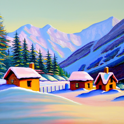
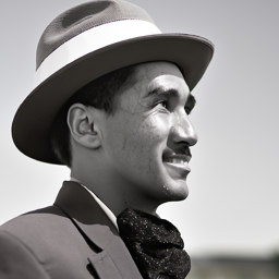
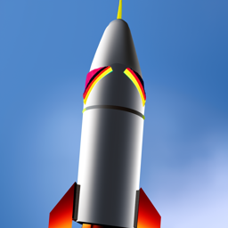
Stage 1: num_inference_steps = 100; Stage 2: num_inference_steps = 20

Stage 1: num_inference_steps = 100; Stage 2: num_inference_steps = 100

Overall, using different num_inference_steps values would results in different images at Stage 1, but the results of the image generation and the values do not seem to have direct correlation. In stage 2 a larger num_inference_steps results in a more detailed image output

1: Sampling Loops

1.1 Implementing the forward process

A key part of diffusion is the forward process, which takes a clean image and adds noise to it. In this part, we define \(t \in [0, 999]\) and computing \(x_t = \sqrt{\bar{a}_t}x_0 + \sqrt{1 - \bar{a}_t}\epsilon \) where \(\epsilon \) is noise sampled from \(N(0,1)\). By this formula, \(t = 0\) corresponds to a clean image, and larger \(t\) corresponds to more noise.

Here are the test image at different noise level:

1.2 Classical Denoising

The classical method is applying Gaussian blur filtering to each image, trying to remove the noise. Obviously, the result dosen't turn out well.

1.3 Implementing One Step Denoising

Here, we use a pretrained diffusion model stage_1.unet to denoise. The model estimate noise in the noisy image. Then we remove the noise to obtain an estimate of the original image by using the above formula to work backwards. \(\hat{x}_0 = (x_t - \sqrt{1 - \bar{a}_t} * \hat{\epsilon}) / \sqrt{\bar{a}_t} \)

1.4 Implementing Iterative Denoising

In part 1.3, we observed that the UNet excels at projecting noisy images onto the natural image manifold, though performance naturally declines as noise increases. However, diffusion models are designed to denoise iteratively. In this part, instead of walk through all 1000 timesteps(which would be computationally expensive), we implemented a faster approach by selecting a subset of timesteps and jumping at regular intervals (e.g., a stride of 30).

Transition Between Timesteps Process:

On the i-th step, we denoise from t = strided_timesteps[i] to t' = strided_timesteps[i+1]. This is governed by the following formula:

\[ x_{t'} = \frac{\sqrt{\bar{\alpha}_{t'}} \beta_t}{1 - \bar{\alpha}_t} x_0 + \frac{\sqrt{\alpha_t} (1 - \bar{\alpha}_{t'})}{1 - \bar{\alpha}_t} x_t + v_\sigma \]

Where:

• \(x_t\): the noisy image at timestep \(t\),
• \(x_{t'}\): the less noisy image at timestep \(t'\),
• \(\bar{a}_t, \bar{a}_{t'} \) : cumulative products of the alphas, related to noise variance,
• \(x_0\): our current estimate of the clean image, obtained using a UNet,
• \(v_{\sigma}\): additional random noise

1.5 Diffusion Model Sampling

By setting i_start = 0 and passing in some random noise, we can get sampled images from the model. Here are some results:

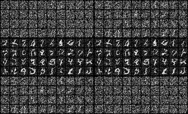
As we can see, most of the generated images are blurry and gray.

1.6 Classifier-Free Guidance (CFG)

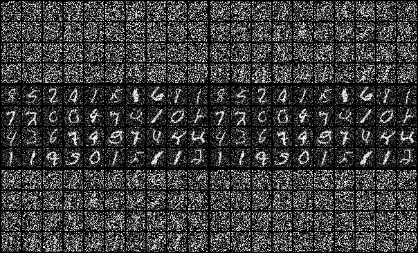
In order to greatly improve image quality, we can use Classifier-Free Guidance, in which we compute both a conditional noise estimate \(\epsilon_c\) and an unconditional noise estimate \(\epsilon_u\). Then, the new noise noise estimate is: \[ \epsilon = \epsilon _u + \gamma (\epsilon _c - \epsilon _u )\] where \(\gamma \) controls the strength of CFG. When \(\gamma > 1\), we magicly get higher quality images. Here are some sampled image with CFG using \(\gamma = 7\):

1.7 Image-to-image Translation

The denoising process effectively allows us to make edits to existing images. The more noise we add, the larger the edit will be. To visualize this kind of editing, here are 3 group of images that get by using the given prompt "a high quality photo" at noise levels [1, 3, 5, 7, 10, 20]

For the simpler image like Campanile, the images start to look similar to the input from i_start= 5, while the more complex images start to show similarity from i_start= 10.

1.7.1 Editing Hand-Drawn and Web Images

Now we start with hand-drawn or other non-realistic images and see how they can get onto the natural image. However, in my perspective, it seems not work very well.

Image from the web:

Hand drawn images

1.7.2 Inpainting

We can use run the diffusion denoising loop to implement inpainting. Given an image and a binary mask, we can create a new image that inside mask area have new content and outside keep the same. The implementation is that after each step, we reset the pixels as where the mask is 0 and add correct noise to them: \[ x_t = mask * x_t + (1 - mask) * \text{forward}(x_{orig}, t) \]

1.7.3 Text-Conditional Image-to-image Translation

In this part, we will do the same thing as SDEdit, but control the output with text prompt "a rocket ship" instead of using the defult setting "a high quality photo". Influnced by both input image and text, the images should look like original image and also look like the text prompt. And with i_start growing, it should look more like the input image, while keeping the text information.

1.8 Visual Anagrams

In this part, we create optical illusions with diffusion models. The illusionary image looks like one text promot, but when flipped upside down will looks like another. The algorithm is:

1. Denoise image \(x_t\) at step \(t\) with the prompt \(p_1\), to obtain noise estimate \(\epsilon_1\).
2. Flip \(x_t\) upside down, then denoise with the prompt \(p_2\), to obtain noise estimate \(\epsilon_2\).
3. Flip \(\epsilon_2\) back, and average the two noise estimates.

\[ \epsilon_1 = \text{UNet}(x_t, t, p_1) \] \[ \epsilon_2 = \text{UNet}(\text{filp}(x_t), t, p_2) \] \[\epsilon = (\epsilon_1 + \text{flip}(\epsilon_2) ) / 2\]

1.9 Hybrid Images

In this part we create hybrid images with a diffusion model by combining low frequencies from one noise estimate and high frequencies of estimate with the other text prompt. \[ \epsilon_1 = \text{UNet}(x_t, t, p_1) \] \[ \epsilon_2 = \text{UNet}(x_t, t, p_2) \] \[\epsilon = f_{low}(\epsilon_1) + f_{high}(\epsilon_2)\]

The image on first line shows the effect of text prompt on low-frequency, while the second line shows high-frequency part with corresponding prompt.

Part B: Diffusion Models from Scratch!

Part 1: Training a Single-Step Denoising UNet

1.1 Implementing the UNet

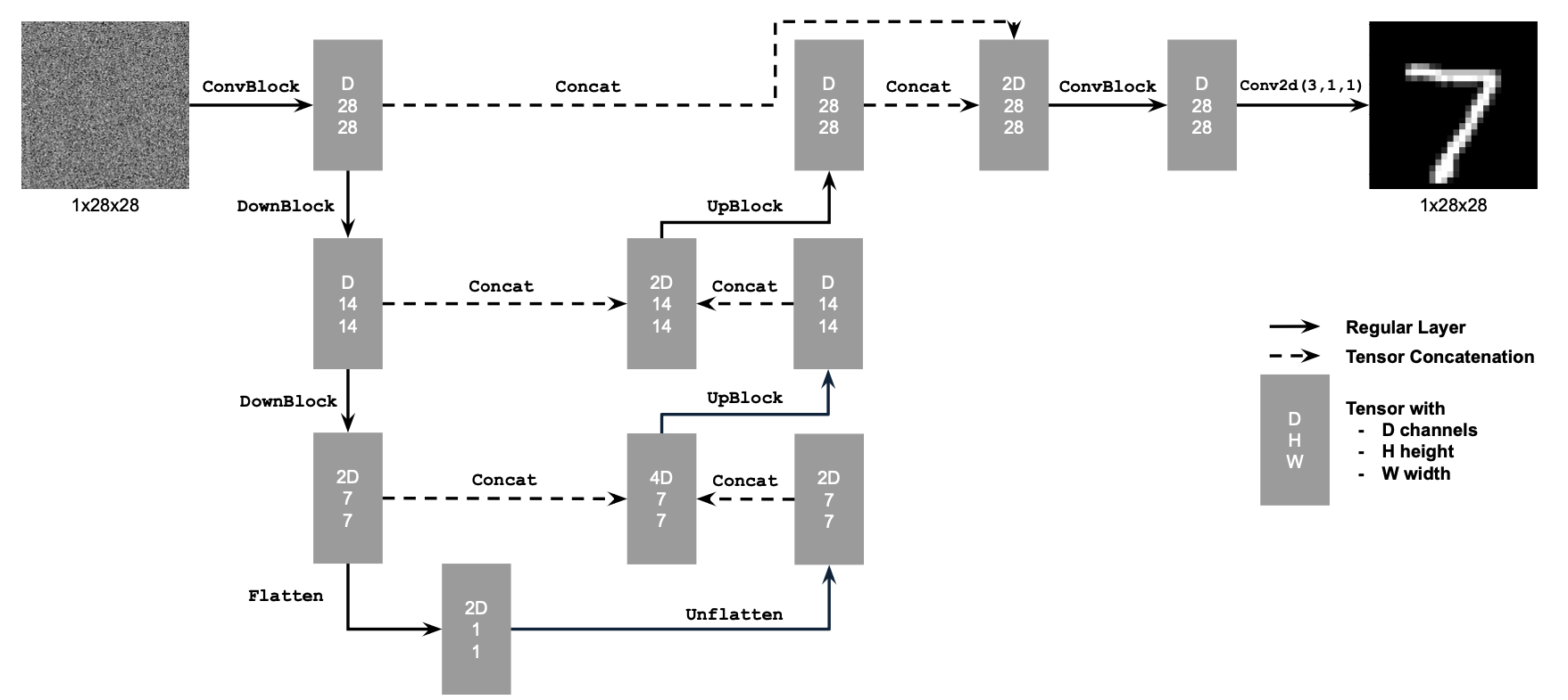
The diagram shows the structure of the Unconditional UNet we implemented:

1.2 Using the UNet to Train a Denoiser

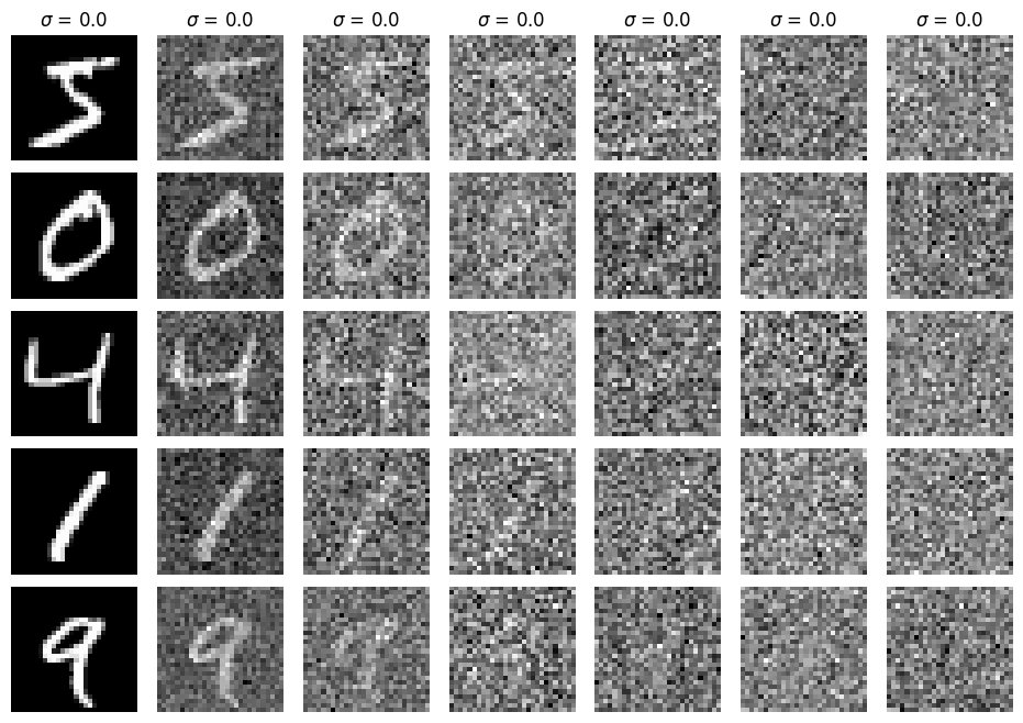
To train our denoiser, we need to generate training data pairs of a clean MNIST digit and a noisy image of digit. We generate the noisy image \(z\) using clean digit \(x\) and \(\sigma \in [0.0, 1.0]\): \[ z = x + \sigma \epsilon, \text{where }~ \epsilon \sim N(0,1) \]

Visualize the different noising processes:

1.2.1 Training

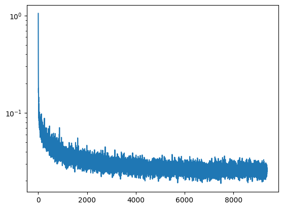
Here are some setting for the training process:

• Noisy level: \(\sigma = 0.5\); Training epochs: 5
• Dataset and dataloader: MNIST dataset with batch size: 256
• Model: Use the UNet architecture defined in section 1.1 with recommended hidden dimension D = 128.
• Optimizer: Use Adam optimizer with learning rate of 1e-4.

1.2.2 Out-of-Distribution Testing

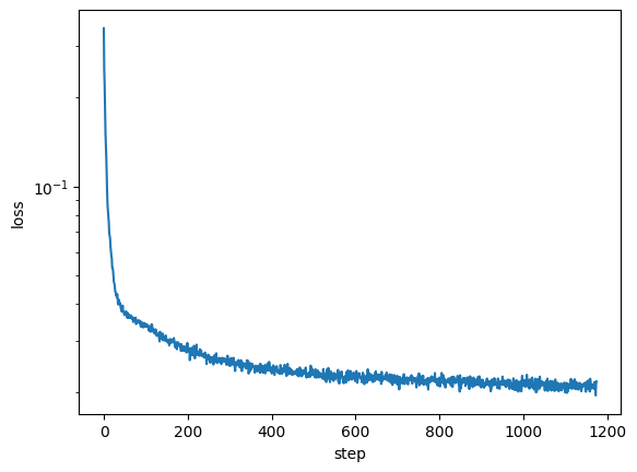
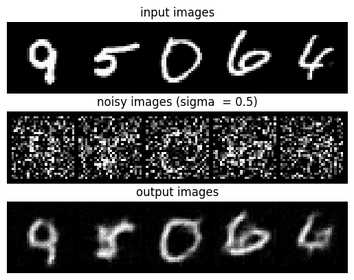
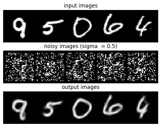
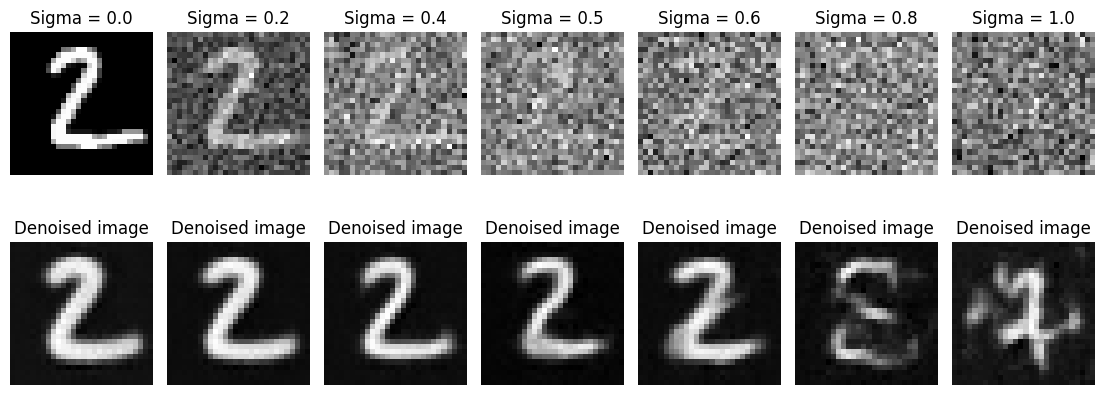
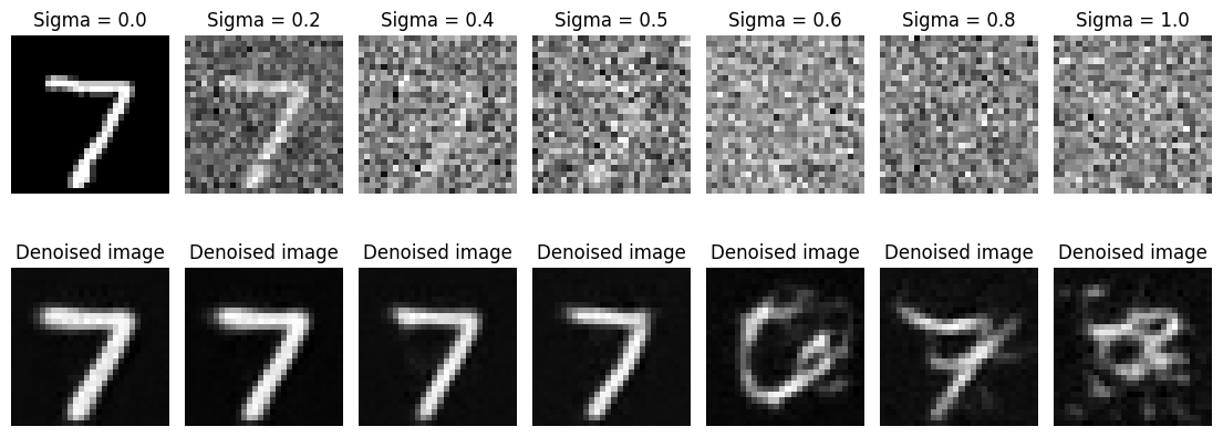
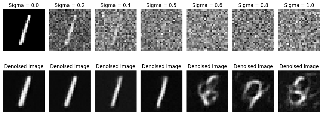
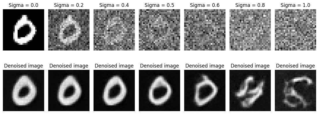
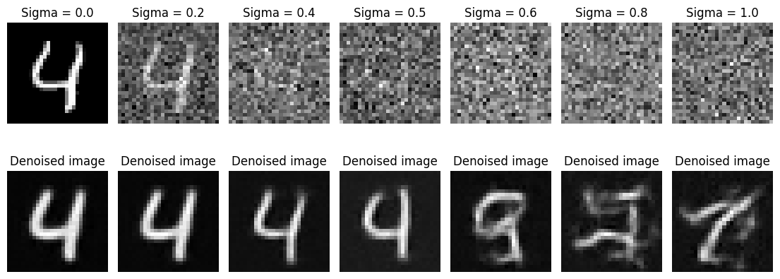
Our denoiser was trained on MNIST digits noised with \(\sigma = 0.5\). Here are visualization of the denoiser results on test set digits with varying levels of noise.

Part 2: Training a Diffusion Model

2.1 Adding Time Conditioning to UNet

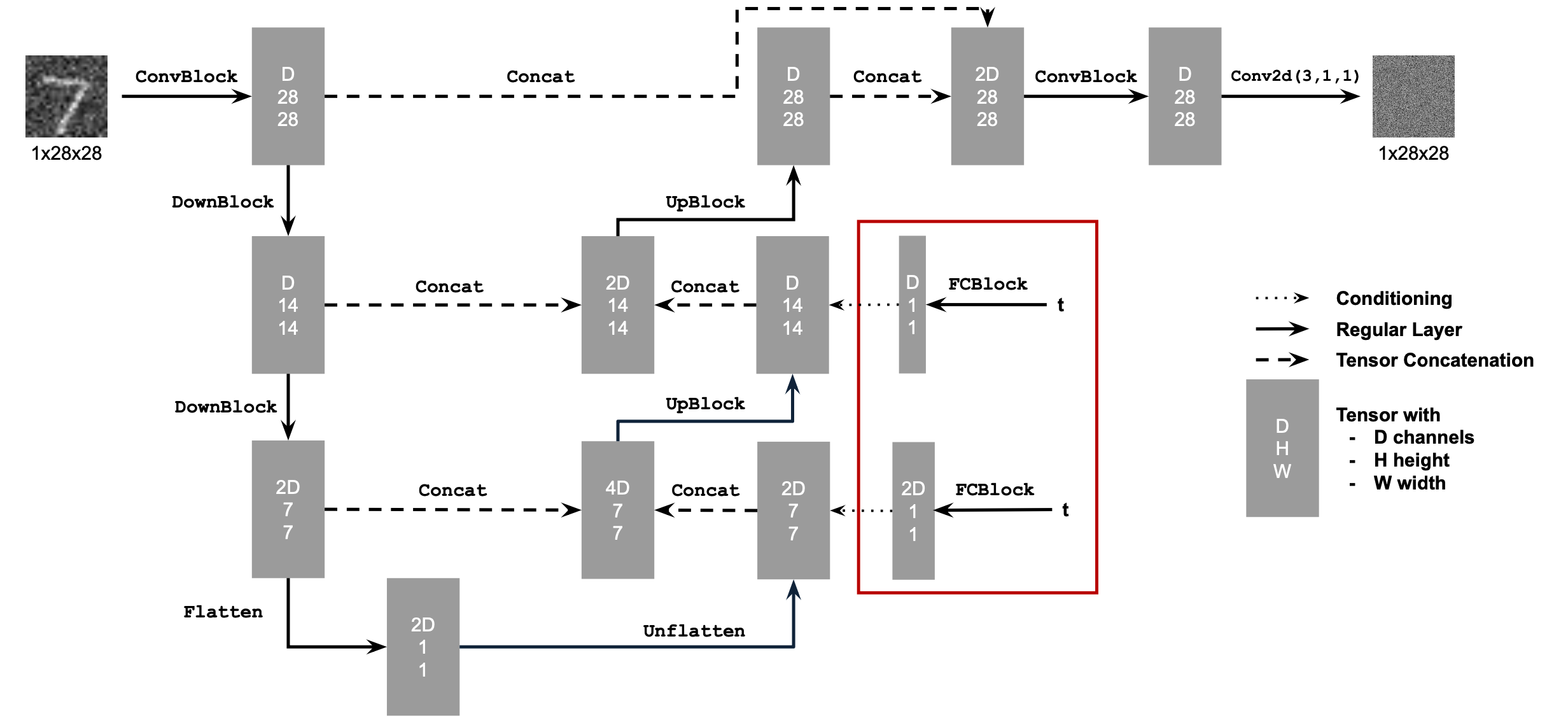
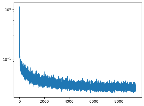
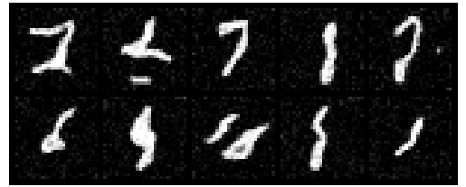
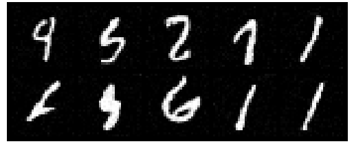
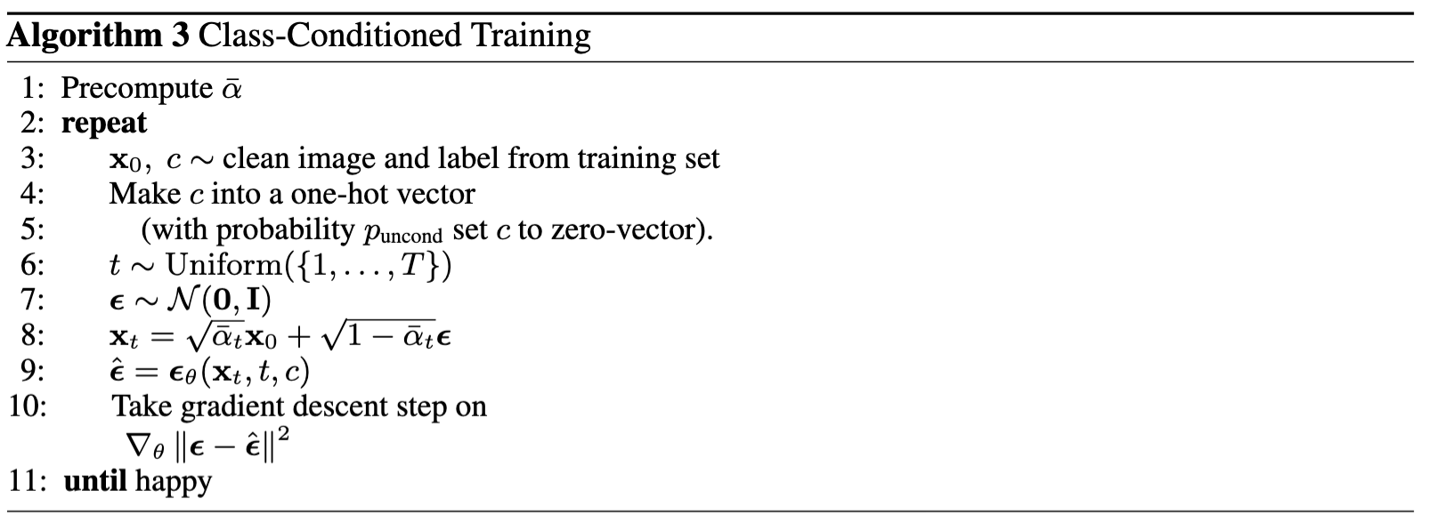
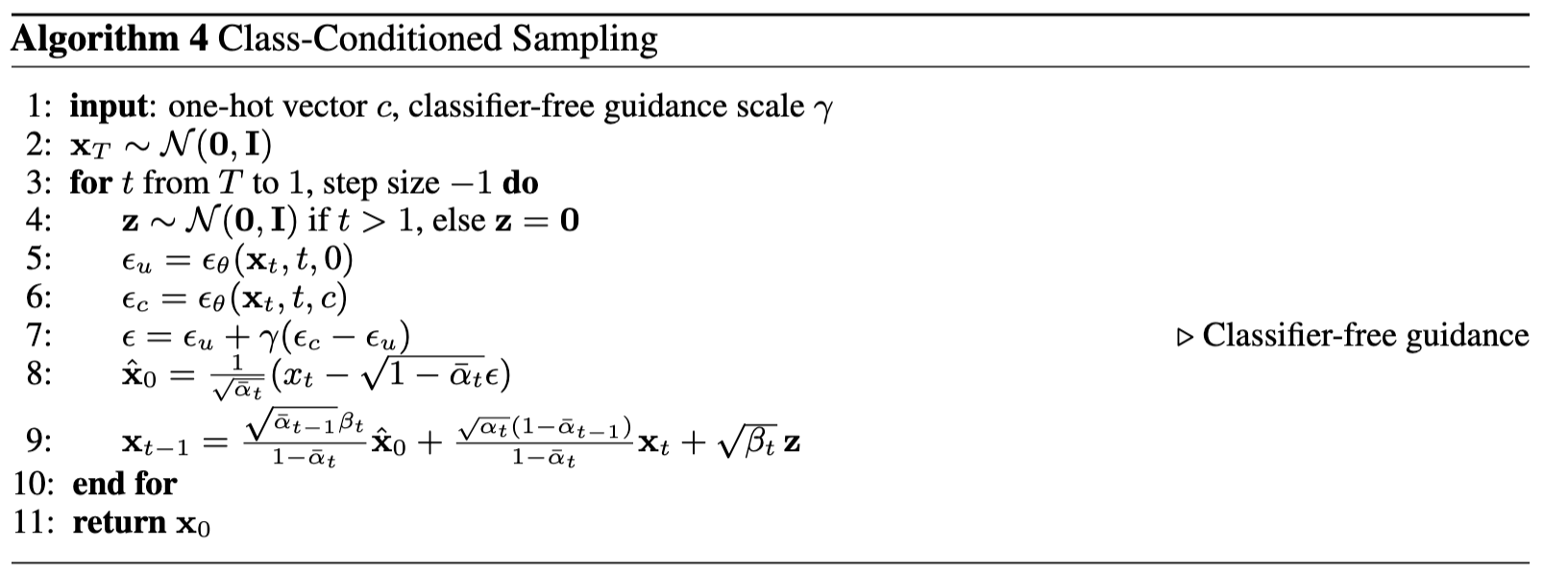
In this Model, we inject scalar \(t\) into the UNet model decoder part to condition.

2.2 Training the UNet

2.3 Sampling from the UNet

2.4 Adding Class-Conditioning to UNet

2.5 Sampling from the Class-Conditioned UNet

Bells & Whistles

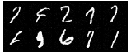
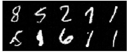
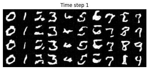
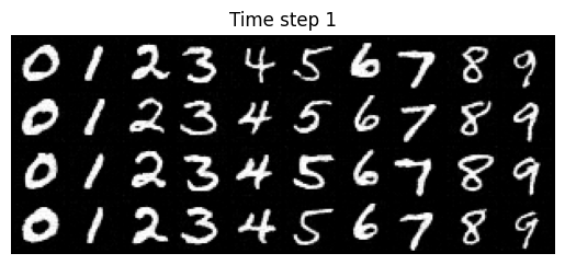
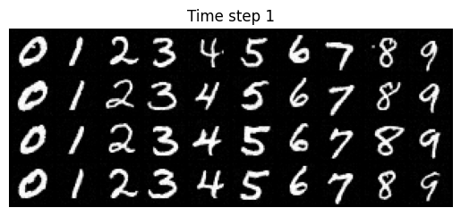
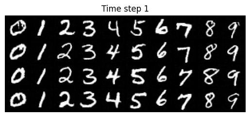
Sampling Gif